Dataset API Configurator

meteoblue offers access to environmental datasets like archived meteoblue weather simulations, ECMWF ERA5, gridded satellite information, soil properties and other reanalysis datasets. The web-interfaces are an easy entry point to:

• Access hundreds of terra-bytes of raw data
• Select single locations or large areas as polygons
• Easy access via web-interfaces and APIs
• Transform data on server side: Filter, aggregate and resample
• Fast. A 30-year hourly data-series can be retrieved within a second
• Run complex calculations with job queues

All data can be retrieved with an interactive web-interface. The user can select a location, time-range, dataset and weather variables. Data can then be downloaded in various formats like CSV, XLSX, JSON or netCDF, but also analysed with interactive charts and maps.

With the concept of transformations, data can be modified easily to get the desired result instead of large amounts of raw data. Examples:

• Aggregate the precipitation amount of a 50-day time-interval
• Resample ERA5 to a 0.1° plate-carree grid
• Calculate the average temperature weighted by a cropland fraction
• Find consecutive frost, heat or excessive precipitation periods

All functionality is available via APIs and can be integrated into other systems.

Web-Interface

The interactive web-interfaces guide users to quickly select desired data from large datasets. They are online to meteoblue customers: https://www.meteoblue.com/en/weather/api/datasetapi. For more information please contact [email protected].

To query data a few simple steps are required:

• Select units for temperature or velocities
• Select locations, coordinates, administrative areas or draw your own polygon
• Select a time interval. E.g. 30 years of data
• Select a dataset and variable: ERA5 temperature on 2 meters above ground
• Visualize as chart or download as XLSX format

Each step is explained below in more detail with caveats that describe what exactly is happening.

Units

Many datasets store wind-speeds in meters per second (m/s) or use different units. To unify access to data, conversions are automatically applied. Celsius (°C), kilometers per hour (km/h) and metric length units are selected as default. The unit-conversion will now show all available wind speed data in km/h.

Coordinates and Polygons

Environmental datasets have different resolutions and grid systems. Some datasets may use regularly spaced 0.5° Gaussian grid. More complex datasets use irregular grids like Arakawa or reduced Gaussian grids. The API and web-interfaces abstract this complexity from the user and allow simple calls with WGS84 latitude and longitude coordinates as well as whole areas using polygons.

The web-interface offers 6 different selection modes:

• Location search: Search for places by name
• Coordinates list: A CSV text input for coordinates
• Coordinates and time: A CSV text input for coordinates and time-intervals
• Daw polygon: A interactive map to draw a rectangle or polygon
• Political area: Select administrative areas from a database
• JSON: Insert a GeoJSON geometry as text

Location Search and Coordinates

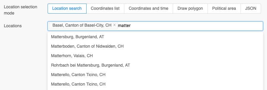
The location search only translates location names to coordinates. Underneath only coordinates are used.

For each coordinate, the system searches for the best-suitable grid-cell of a dataset. For complex terrain this might not be the closest grid-cell. If the user calls data for a location in a valley, the nearest grid-cell could be on a mountain with significantly higher elevation. The system automatically searches surrounding grid-cells to find a grid-cell which might also be in this valley. Grid-cell on sea are also avoided, because they have characteristically different weather properties.

It is important to understand, that grid-cells do not have a perfectly defined spatial extend and that higher resolution does not necessarily improve data quality. Higher resolution could actually lead to poorer data quality.

In the later examples we show options to arbitrarily increase the resolution of a dataset, but we highly recommend using single coordinates and let the API decide which grid-point to select.

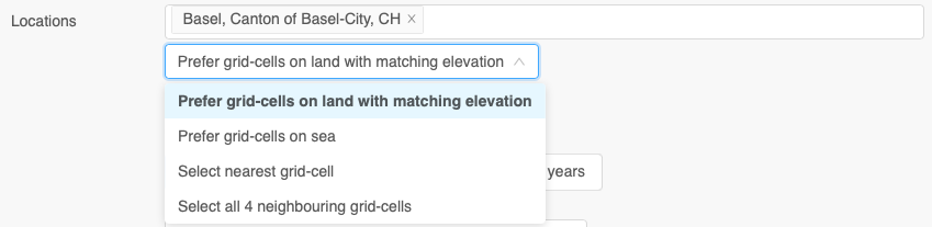
For more fine grained control, different grid-point selection modes are available:

• Prefer grid-cells on land with matching elevation: Selects the best suitable grid-cell for a selected location. Grid-cells on land are preferred and analysed to match elevation with the selected location.
• Prefer grid-cells on sea: Selects a close by grid-cell on sea. This is helpful to display weather forecasts on sea with stronger wind characteristics.
• Select nearest grid-cell: Simply select the closest grid-cell. This can be counter intuitive, because grid-cells with sea characteristics can be selected at coastal areas.
• Select all 4 neighbouring grid-cells: Returns 4 closest grid-cells for each selected location. This can support machine learning applications to detect and predict small scale spatial patterns.

Coordinates List

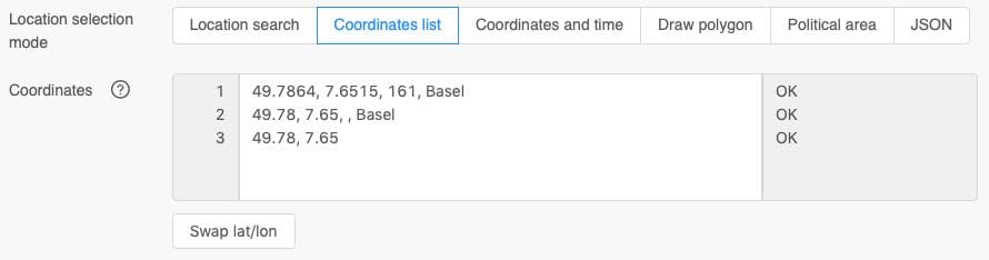
As an alternative to the location search selection, a list of coordinates can be used. The interface expects a comma separated list of latitudes, longitudes, elevation and a location name. Tabs and white spaces are also accepted as separator and detected automatically.

Coordinates must use the latitude and longitude WGS84 decimal degrees notation like -47.557 6.8115. Coordinates in the sexagesimal notation with hours and minutes like 47°33'25.2"S 6°48'41.4"E are NOT accepted. Please be careful to correctly convert from sexagesimal to decimal degrees notation.

Elevation and location names are optional. If the elevation is unknown, a digital elevation model (DEM) with 80-meter resolution is used automatically. The location name is only used in the output formats and graphs to make it more readable.

There is no fixed limit on the number of coordinates, but the web-interfaces struggle with more than 25000 coordinates. The API may also refuse too many coordinates, because the upload size of the coordinates list is limited to 20 MB. If you want to process more coordinates, please split them in chunks of a few thousands at once.

Coordinates and Time

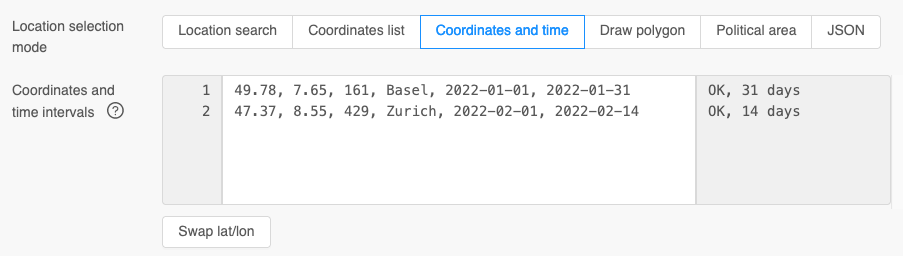
For certain use-cases for each coordinate a different time-interval can be selected. This is handy if there is an existing spread sheet with time-intervals and coordinates.

The interface expects a comma separated list of latitude, longitude, an optional elevation and an optional location name. Additionally, a start and end date is required. The dates must be ISO8601 (YYYY-MM-DD) formatted.

With copy&paste the coordinates and time-interval list can be transferred to the interface. Please make sure to use the correct columns and keep empty columns in case elevation or location name is missing. In the image above tabs are used. It is not apparent to the eye where tabs and white spaces might be.

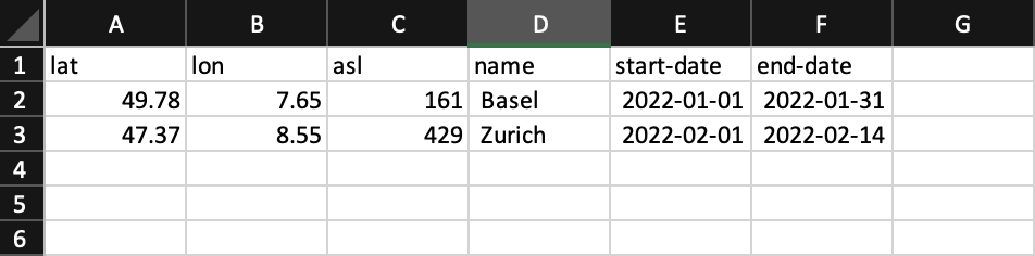
Spread sheet applications commonly use tabs as a separator while coping. The following comma separated list produces the same result.

49.78,7.65,161,Basel,2022-01-01,2022-01-31     // lat, lon, asl
47.37,8.55,429,Zurich,2022-02-01,2022-02-14     // lat, lon, asl

Draw Polygon

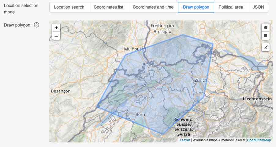
To select data from all grid-cells in a given area, polygons can be drawn in the interface. The 3 buttons in the right side of the map start the drawing for a polygon or a rectangular box. Polygons can also be edited.

The API will now extract all grid-cells where the grid-cell center is inside the drawn polygon. Grid-cells do not have a proper spatial extend and intersected grid-cells are not included. There is also no exclusion of sea-points or any height adjustment. If you are using small polygons that barely include any grid-cells, consider using regular coordinate calls.

The following map shows temperature values from grid-cells in the meteoblue NEMS4 high-resolution domain for Switzerland. The small colored dots are centered on each grid-cell center and do not represent the spatial shape of a grid-cell.

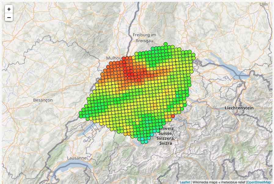
The size of a polygon is not limited, but very large polygons at continent level may take several minutes to extract data. This depends on the resolution of the dataset. A fine-grained dataset with 250-meter resolution may include millions of grid cells, but a 25 kilometer global dataset includes only a couple of hundreds for the same area.

Political Area

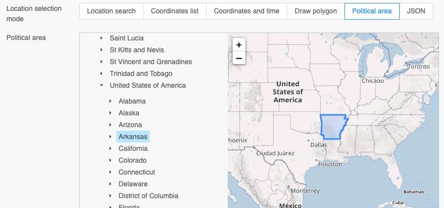
Commonly whole countries or administrative areas are analysed. The web-interface and APIs include a database with political areas to simplify the process. Political areas follow the same behaviour as polygons and only include grid-cells which grid-cell-centre is inside the polygon.

For smaller regions some polygons might not be available. We recommend using regular coordinate based calls instead.

JSON

The API and web-interfaces use the GeoJSON standard to select points and polygons. The JSON can also be used directly in the web-interface. GeoJSON expects coordinates in tuples of longitude and latitude while the result shows latitude and then longitude.

The GeoJSON syntax is also explained in more detail in the Dataset API documentation

{
  "type": "Feature",
  "geometry": {
    "type": "Polygon",
    "coordinates": [
      [
        [6.8115234375, 47.557993859037765],     // lon, lat
        [7.355346679687499, 46.852678248531106],
        [7.9541015625, 47.331377157798244],
        [7.459716796875001, 48.25394114463431],
        [6.9927978515625, 48.151428143221224],
        [6.8115234375, 47.557993859037765]
      ]
    ]
  }
}

Time-Intervals

Most datasets offer data for multiple years in hourly or daily resolution. After a location or area has been selected the time-interval needs to be specified.

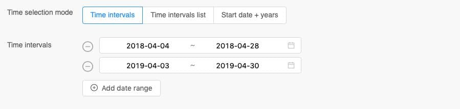
Multiple time-intervals can be selected at once. If 10 locations are selected and 4 time-intervals, the API will provide for each location 4 data-time-series. 40 in total.

A UTC-offset can also be specified. Per default UTC is used +00:00. European wintertime +01:00, European summer time +02:00, Pacific time -07:00 as well as other time-offsets are available. The UTC-offset is important for daily aggregations. For monthly and yearly aggregations, the API will only use UTC time.

There is no support for day-light-saving time. Data can either be extracted as summer or wintertime.

Time Intervals List

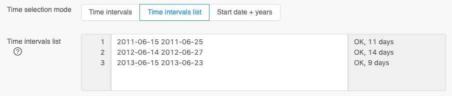
Analog to the coordinates list, a comma separated list can be supplied for time-intervals. The date must be formatted as ISO8601 (YYYY-MM-DD). Other date formats like DD.MM.YYYY or MM/DD/YYYY are not supported.

Start Date + Years

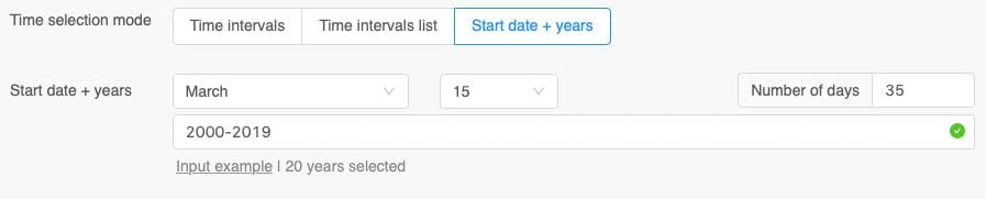
To conveniently compare a time-interval in multiple years, the Start date + years mode can be used. In the image above, 20 years are analysed starting at 15th March for 35 days.

In a leap year, time-intervals covering 29th February will have the same number of days, but the calendric last date will be one less.

Datasets and Weather Variables

Environmental datasets are categorized by type and resolution. The first category Weather/Climate contains ERA5, BOM and Tropical Storms Reanalysis. Weather (1-10 km) groups high-resolution weather simulation domains from meteoblue and national weather services.

A complete list of environmental datasets can be found here.

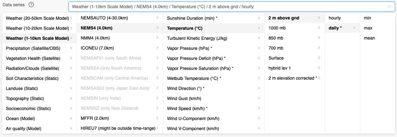
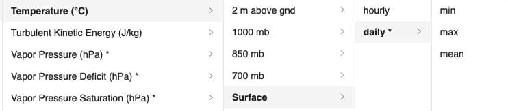
Each dataset contains many weather variables like temperature or wind speed. Each weather variable has usually different levels like 2 meter above ground, surface or 850 hPa.

Each level may contain different time-resolutions like hourly or daily data. Finally, for daily data different aggregations can be selected.

With this cascaded selection process, hundreds of weather variables on different levels and time-resolutions are available. The list can be searched for keywords like Clay to quickly find datasets containing information about clay.

Some weather variables are marked with an asterisk like Wind Speed (km/h) *. This means they are derived variables that are computed using other variables available in this dataset. As an example, datasets typically store U and V wind components instead of wind speed. With a simple $v = \sqrt{u^2 + v^2}$ calculation wind speed can be derived. More complex models like FAO Reference or leaf wetness probability are also available as derived variable. A more detailed list of derived variables can be found in a later section.

Weather variables are available on different levels. Temperature is typically measured and simulated at 2 meter above ground. Wind measurements use 10 meter and 80 meter above ground levels. Soil datasets use different depth layer below surface. Some levels can also be derived from others: A special 2 m elevation corrected * level is used to adjust the temperature of the grid cell to requested elevation using a lapse rate. Levels like hybrid lev 1 are specific to a dataset and described in more detail at the dataset documentation.

As a last step the time-resolution and aggregation can be selected. Most datasets use hourly or 3-hourly time-resolution. As before an asterisk marks time-resolutions that are calculated automatically. daily aggregations for example are frequently used and offered directly as derived time-resolution. Time resolutions like monthly or yearly can be calculated with transformations (see below). Datasets that do not offer time-series data like soil characteristics show a time-resolution as static.

Transform Data

Commonly environmental data needs processing to fulfill a certain task. E.g. calculate heat stress indices for a region or build a precipitation sum. The web-interfaces and APIs offer this functionality to perform complex calculations direct on the meteoblue server infrastructure instead of downloading huge data files, reading them and processing them manually.

Multiple transformations can be chained together and are processed one-by-one in the same order whereby the result of the first transformation is input into the next transformation. In the following example hourly temperature from ERA5 from the year 2018 is used and three transformations:

• Resample to a 0.1° grid using linear interpolation
• Search for values greater than 30°C and use 0 or 1
• Aggregate the whole 1-year time interval to a total sum

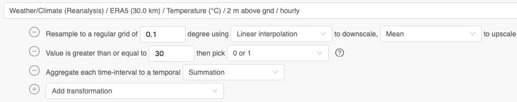
The result is the total number of hours above 30°C within one year based on a down scaled ERA5. For the area around Basel, this would generate the following map. In 2018 there were 195 hours above 30°C in Basel. Data can of course be downloaded as CSV or XLSX data formats.

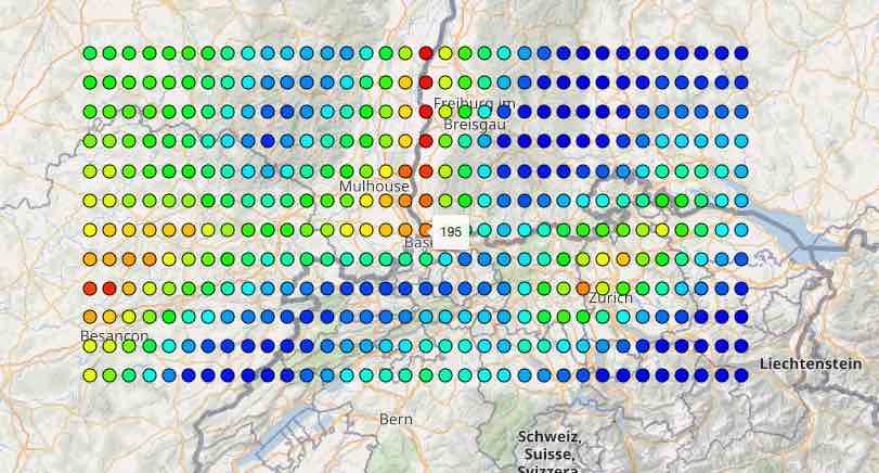
Transformations may heavily modify data while the resulting chart or CSV file may still show Temperature [2m] although ERA5 has been down scaled to a 0.1°. Please be careful how you handle and further communicate data. We carefully store data as "raw" and unmodified as possible.

Reading and transforming data may take some time. Long time-intervals on larger areas with high-resolution datasets quickly require a couple of gigabytes of memory. More complex jobs will be executed in the background on a job queue. Unfortunately, due to the complexity of many calculations, it is very hard to forecast how much time it takes. We recommend running API calls on a smaller geographical extend first and then increase the area.

The concept of transformations is incredibly flexible, and we constantly implement additional transformations. Many complex use-cases can be modeled with transformations. In the chapters below, you will find additional explanations for each transformation.

Gap-Filling

Environmental data may contain a lot of missing values. Satellite precipitation datasets commonly have a first run with a delay of a couple of days and a lot of missing values, until the final run arrives and replaces most missing data. Other datasets like ERA5 offer no real-time updates or forecasts.

To automatically fill missing values with another dataset we implemented a gap-filling process. Example:

• If you select a temperature series from 2000 until today, the most recent data will be missing
• If Fill gaps with NEMSGLOBAL is selected, the most recent data will be provided by NEMSGLOBAL

The gap-fill process calculates the bias between both domains and uses a best linear unbiased estimator (BLUE) to adapt the gap-filled values to the original dataset. Bias correction is only used for temperature, dew point and wind speeds. Other variables are not bias corrected.

We highly discourage the use of gap-filling for machine learning. These algorithms may be sensitive to changes in bias. If you require consistent data of the past 30 years with 7 days forecast, select NEMSGLOBAL directly.

Internally gap-filling is an early action that happens before any variables are derived or transformations are applied. Gap-filling is an expensive operation that may increase the run-time of a data call significantly.

Formats

The web-interface and APIs offer various output formats like CSV, XLSX, JSON, GeoJSON maps or NetCDF files. Formats like CSV and XLSX offer different flavours optimized to larger temporal extend or larger time-intervals.

Charts

For a quick visualization the web-interface use dynamic charts that interactively show long time-series. This makes working with larger datasets quite easy. When you are building complex calls with transformations, it is easier to test your transformations one a single location, visualize a graph and then switch for larger geographical area.

Charts aggregate data automatically to be able to display it. A 10 years hourly time-series contains almost 100'000 data-points and computer struggle to paint a chart with so much detail. Instead, the charts automatically build daily, weekly or even monthly aggregations. In the preview below hourly data are automatically aggregated.

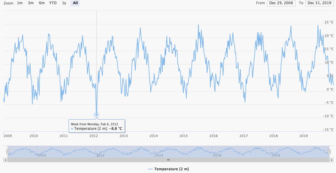
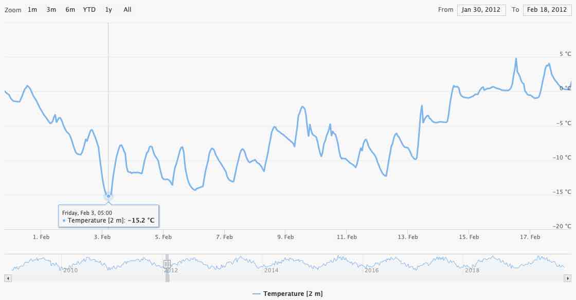
A single day with -8.8°C is clearly visible on Monday 2020-02-06. Beware, the -8.8°C is aggregated and may not be the global minimum in this time-series. Once you zoom in the graph, you see that the minimum temperature is actually -15.2°C on Friday 2020-02-06.

Charts are limited to 100 locations. More data-series tends to significantly slow down your web-browser.

Realign Time Axis

You can realign the time-series in case you want to compare multiple growing seasons. In the next example growing seasons starting on March 1st for the years 2016-2019 have been selected. The graph treats them individually.

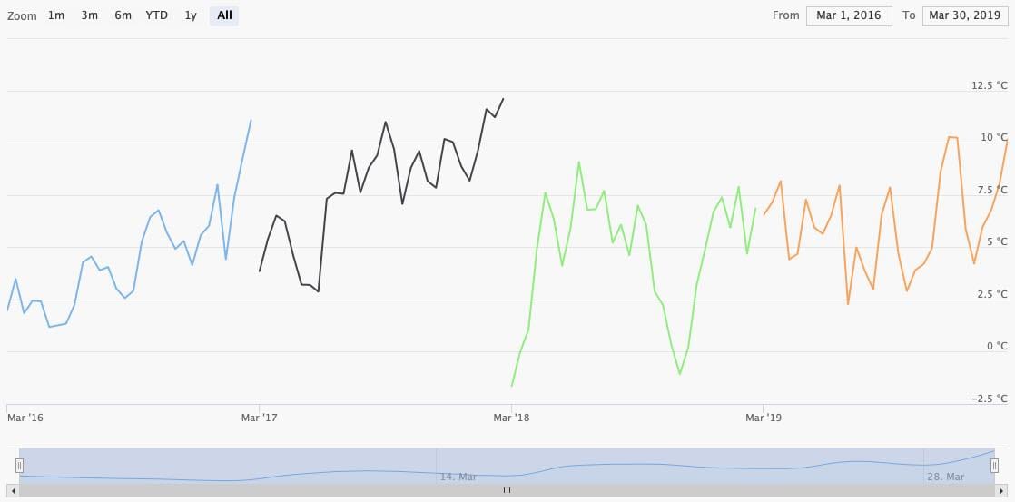
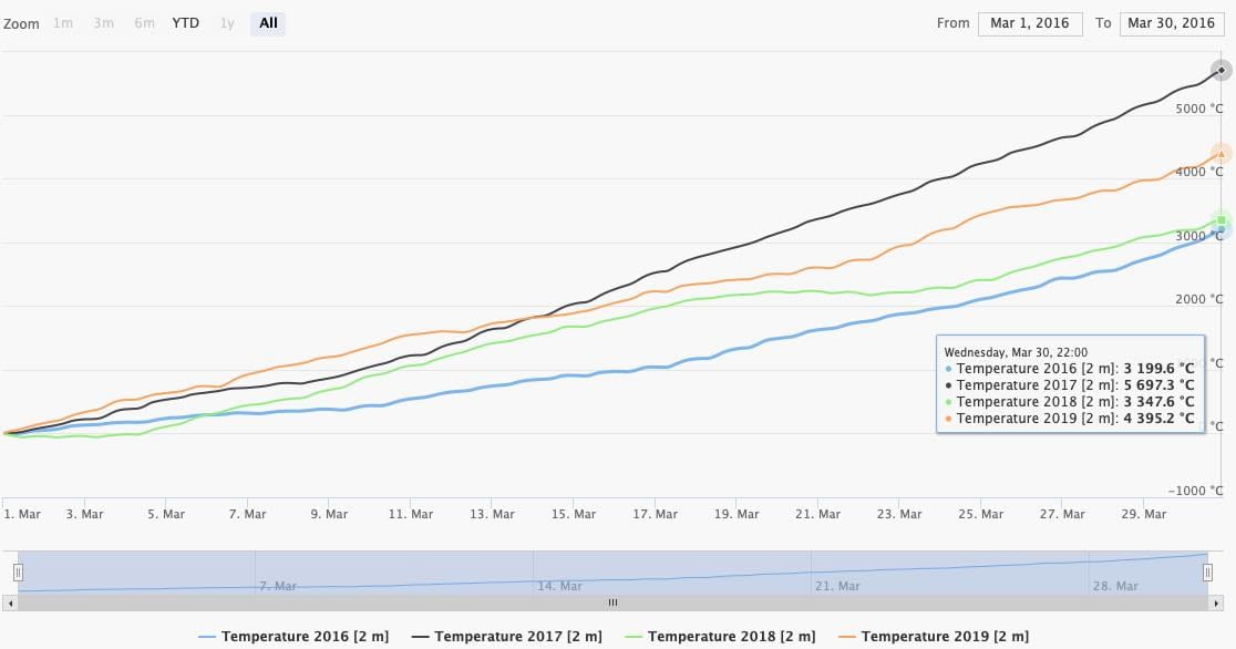
Setting Align intervals in chart to Same start year realigns every graph to a common start date. In combination with the transformation Accumulate time-series to a running total we can create a chart with accumulated temperatures for easy comparison.

Maps

For a quick spatial overview of data, a simple map with markers can be generated. Only the first time-step is considered. The color scales automatically from blue to red.

When using the API directly, you could use the resulting GeoJSON to generate your own map plots.

CSV and XLSX

CSV and XLSX can be used to open the result in Office applications. Especially for Microsoft Excel we recommend using XLSX directly, because importing CSV files may detect decimal separators and date times differently.

Both formats are limited in a way they support structured data or multi-dimensional data. For CSV and XLSX three different options are available with different ways of how the data are structured:

1. Regular: Rows are used for locations; Columns are used to time-steps. This works well for a lot of locations, with few time-steps
2. For long time series: Rows are used for time-steps and columns for locations. This is optimized for very long time-series
3. For irregular time series: Rows are used for time-steps and locations. Columns just consists of a single Value column. This works well for the coordinate selection mode Coordinates and time explained before

CSV and XLSX formats are very inefficient for large datasets, because numeric values are stored as text with a lot of overhead. This may result in a failed call because the file is too large, or the file cannot be opened anymore in Office applications. You could try to use transformations to aggregate data to a lower temporal or spatial resolution.

For larger datasets, please consider NetCDF (or at least JSON).

JSON

JSON format is preferred to integrate the API into other systems. It resembles closely how data are processed internally and is relatively efficient to transfer.

There is one JSON format that has to fulfill a multiple of requirements that resemble the how the JSON is structured:

• Multiple dataset and each dataset may return different grid-points
• Multiple time-intervals
• Multiple weather variables might be read per dataset

The following JSON is returned for hourly NEMSGLOBAL temperature data-series for Basel and Zurich:

[ 
   { 
      "geometry":{ 
         "type":"MultiPoint",
         "locationNames":[ 
            "Basel",
            "Zurich"
         ],
         "coordinates":[ 
            [7.5, 47.66652, 499.774],     // lon, lat, asl
            [8.4375, 47.33319, 549.352]     // lon, lat, asl
         ]
      },
      "timeResolution":"hourly",
      "timeIntervals":[ 
         ["20200101T0000","20200101T0100","20200101T0200",...]
      ],
      "domain":"NEMSGLOBAL",
      "codes":[ 
         { 
            "code":11,
            "variable":"Temperature",
            "unit":"°C",
            "level":"2 m above gnd",
            "aggregation":"none",
            "dataPerTimeInterval":[ 
               { 
                  "data":[ 
                     [0.77,1.27,1.51,1.51,1.32,0.95,0.34,...],
                     [2.32,4.51,6.52,8.34,10.03,11.6,13.09,...]
                  ],
                  "gapFillRatio": 0
               }
            ]
         }
      ]
   }
]

Because only one dataset is selected, the outer array contains one structure. This "per domain" structure has the attributes geometry, timeResolution, timeIntervals, domain, codes:

• geometry lists the selected grid-points as GeoJSON. The coordinates point to grid points with elevation and not the requested coordinates. Basel is actually at 47.56°N/7.57°E with an elevation of 279 meters, but the output shows 47.67°N/7.5°E at 499.78 meters. The grid point has been selected by a nearest neighbor match. The order of arrays is strictly preserved! The first requested location will also be the first returned grid-cell.
• timeIntervals list multiple time-intervals if requested. In this example only one time-interval is present stating on 20200101T0000. With an hourly timeResolution.
• codes will now contain an array of structures for each requested weather variable code e.g. temperature or precipitation.

The "Per weather code" structure contains the attributes code, variable, unit, level, aggregation and dataPerTimeInterval:

• code is the numeric identifier for a weather variable. E.g. 11 for temperature.
• unit is the returned unit for this weather variable after unit conversions or transformations.
• level indicates the height or elevation for this variable. 2 m above gnd is common for temperature.
• aggregation shows min/max/mean in case of temporal aggregations are used. The aggregation for spatial transformations is not shown here.
• dataPerTimeInterval is now an array with a structure for each time-interval. In this case only one.

The "Per time interval" structure contains the attributes data and gapFillRatio:

• data is a 2 dimensional array. The first dimension is used for the number of grid-cells (2 in this case). The second dimension is used for the number of time-steps. The data array can be huge!
• gapFillRatio is the fraction from 0-1 of how much data was gap-filled with another dataset in case gap-fill is active.

The JSON format depends heavily on the correct order of arrays. The use of enclosed arrays is a bit tricky to understand but was chosen deliberately to efficiently encode large data arrays with millions of floating-point values.

KML

KML only returns the grid-cell coordinates, but no data. It is solely used to display the locations of grid-cells in Google Earth.

NetCDF

NetCDF is a binary data-format with support for many popular programming languages and is efficient to transfer larger amounts of gridded data. We recommend the use of NetCDF for further analysis with Python or other scientific programming languages.

The APIs and web-interfaces generate compressed NetCDF4 files based on HDF5 that can be read by any NetCDF or HDF5 reader. In the following export of 1-year temperature data for 8 locations, the NetCDF file contains:

• Spatial dimensions x, y and a temporal dimension time
• lat and lon coordinate float arrays
• time integer64 array which contains signed 64 bit unix timestamps
• A data array for each weather variable. In this case Temperature with attributes about unit, level and aggregation

# ncdump -h dataexport_20200131T094150.nc
netcdf dataexport_20200131T094150 {
dimensions:
	x = 8 ;
	y = 1 ;
	time = 8760 ;
variables:
	float lat(x, y) ;
		lat:_FillValue = NaNf ;
	float lon(x, y) ;
		lon:_FillValue = NaNf ;
	float asl(x, y) ;
		asl:_FillValue = NaNf ;
	int64 time(time) ;
		time:_FillValue = -999LL ;
		string time:resolution = "hourly" ;
	float Temperature(x, y, time) ;
		Temperature:_FillValue = NaNf ;
		string Temperature:unit = "°C" ;
		string Temperature:aggregation = "None" ;
		string Temperature:level = "2 m" ;

// global attributes:
		string :domain = "NEMSGLOBAL" ;
}

API Call

The web-interfaces retrieve all data from APIs. Internally they build an API call syntax and then execute it. Because of the use of transformations, various geographic and temporal context, the API call syntax is complex and harder to understand.

To quickly build an API call, we recommend using web-interfaces and the generated calls. The API syntax is explained in more detail in the next document for the dataset API.

Reuse Calls: Share Strings

To save and restore all configurations in the web-interface, the Reuse call menu offers the option to Generate share string. This string can be shared with colleges or saved for later use.

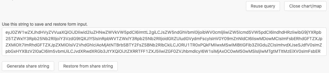
Note: Older share strings may be incompatible, because of changing features in the web-interfaces

Derived Variables

Many datasets store only a small portion of environmental and weather variables, because many variables can be derived from other variables. Commonly weather forecast datasets only store U and V wind components instead of wind speed and direction. The web-interfaces and APIs calculate derived variables on demand.

Derived variables are marked with an asterisk in the dataset and weather variables selection. Not only weather variables are derived, but also levels and time resolutions.

Trivial derived variables:

• Relative humidity from temperature and dew point
• Wind speed and direction from U/V wind components
• Wet bulb temperature from humidity and temperature
• Snow fall amount: Precipitation and snow fraction
• Daylight duration solely based on time a location
• Sunshine duration based on cloud cover and daylight duration

Implicit Daily Aggregation

Many datasets offer hourly time resolution data, but the use of daily data if often more convenient. The web-interfaces offer for many weather variables a daily aggregation with different methods of aggregations.

Daily aggregations are not offered directly for all weather variables or may not include all aggregations. The APIs support for datasets daily aggregations. In case another aggregation function is required (e.g. standard deviation), temporal transformations also offer the option to aggregate to daily data.

Please make also sure to select a correct timezone offset.

Hourly Interpolation

Some datasets like GFS only offer 3-hourly data. The web-interfaces show an hourly derived time resolution to implicitly interpolate.

Depending on the variable, different methods are used for interpolation:

• Hermite interpolation is used for most variables to interpolate a smooth curve.
• Linear interpolation is used for precipitation and then correctly scaled to preserve the total amount
• For solar radiations a spline interpolation is used in combination with explicitly modeled solar zenith angles.

Temporal interpolations to 1-, 5-, 10- or 15-minute data are also available as an additional transformation.

Two Meter Elevation Corrected

Commonly the 2 meter above gnd level is used for temperature. Because grid-cells may be further away from desired locations and have different elevations, a derived level 2 m elevation corrected is available to adjust temperature to the height difference. A simple 0.65°K per 100m elevation is applied. meteoblue forecast APIs use more advanced techniques to adjust temperatures for locations in complex terrain, but as soon as temporal aggregations exceeds 1 month, a linear correction is sufficient.

The 2 m elevation corrected is only available for calls for individual coordinates, but not for polygon areas. In case the elevation of the requested coordinate is not provided, a digital elevation model (DEM) is used.

Analog to temperature, wind speeds can also be adjusted from the common 10 m above gnd to 2 meter using a logarithmic wind profile. From 10 meters to 2 meters this results in a simple factor of 0.75. Please note that this approach is not suitable to downscale further, because of uncertainties in low level turbulence and roughness and is only valid over tiny vegetation like very short grass.

Growing Degree Days (GDD)

Growing degree days (GDD) with base and maximum temperature parameter can be directly selected as a derived variable in the web-interfaces. GDD can also be calculated for a 2 m elevation corrected level.

GDD is directly calculated from hourly data instead of the less precise approach with daily minimum and maximum temperature. With hourly data, daily temperature variations reflect more accurately in GDD.

$$GDD = \int ((T(t) - T_{Base}) < T_{Max}) dt$$

If Fahrenheit is selected, the GDD calculation expects base and maximum temperature in Fahrenheit and returns GDDf.

For Tmin or Tmax ∉ [Tbase,Tlimit], the growing degree day variable is defined as 0.

Growing Degree days daily min/max

Similar to the Growing Degree Days (GDD) variable above. Except that this variable calculates GDD based on daily minimum/maximum data instead of using hourly data.

Each daily minimum and maximum temperature is bounded to the base and limit temperature before calculation.

$$T_{min}, T_{max} \in [T_{base}, T_{limit}]$$ $$GDD = \frac{T_{max} + T_{min}}{2} - T_{base}$$

Leaf Wetness Probability

We use an experimental approach to model leaf wetness and return probabilities. This model is based on precipitation, heat fluxes, temperature and humidity. This model may work well in combination with machine learning for disease models.

Apparent Temperature

The apparent or felt temperature considers the cooling effect of wind (wind chill) as well as heating effects caused by relative humidity, radiation and low wind speeds. It is based on the formula of Robert G. Steadman but has then been developed further by meteoblue.

Vapor Pressure and Air Density

Vapor pressure is calculated using the Wexler function. Vapor pressure deficit and saturation are calculated accordingly.

Air density calculated from vapor pressure, temperature and humidity.

Cloud Cover Total

The total cloud cover is based on low, medium and high clouds. Different cloud layers weighted accordingly.

Evapotranspiration and FAO Reference

Evapotranspiration is directly derived from latent heat flux.

Furthermore, the FAO reference Evapotranspiration is available. FAO uses the Penman-Monteith method with hourly temperature, wind speed, humidity and shortwave radiation as input. See Reference Evapotranspiration (Eto)

Photosynthetic Active Radiation

Photosynthetic Active Radiation as well as photosynthetic photon flux density are based on shortwave radiation.

ERA5 Soil Moisture Classes

In ERA5 soil moisture saturation, residual, field capacity, wilting point, capacity available to plant at field capacity are based on the ERA5 texture class and offer only one static value.

Soil moisture available to plant and transpirable fraction use texture classes in combination with hourly soil moisture.

Diffuse Short-Wave Radiation

Some weather datasets offer diffuse radiation directly. In case it is not available, it is calculated based on short-wave radiation according to Reindl.

Tilted Short-Wave Radiation

The global irradiation on a tiled plane (GTI) can be calculated as a derived parameter. GTI is used for photovoltaic panel power production and based on short-wave and diffuse radiation as well as the zenith and azimuth angle of the sun. Diffuse radiation of a data-set will be used directly if available, otherwise Reindl is used.

In case a gap-fill dataset is selected, GTI would be calculated independently for both datasets and afterwards merged together.

The calculation considers the backwards averaged levels Surface and 5x5@sfc as well as instantaneous values for the level instant@sfc.

Two parameters are required:

• slope: The inclination of the panel relative to ground. Commonly this is 20°. 0° would be horizontal to the ground; 90° vertical.
• facing: The east-west facing of the panel. Commonly faced towards the south at 180°. 90° = East, 180° = South, 270° = West.

More information on solar energy calculation is available here.

Shortwave Radiation: Instant and 5x5 Levels

Typically, shortwave radiation is backwards averaged in weather models. For hourly data the value at hour 16:00 is an average from 15:00 until 16:00. Measurements often report the value at exactly that hour.

A clear data offset is visible in the data. To correctly compare data, we adjust backwards averaged radiation to a value at this instant. This adjustment is not trivial, because the correct sun zenith angle must be considered.

The level 5x5@sfc is available for solar radiation variables for certain datasets and is an averaged value of the surrounding 5x5 grid-cells. In certain situations, this yields better results with machine learning than using a value of only one grid-cell.

Aggregated Soil Depths

The SOILGRIDS dataset offers soil variables at depths 0, 5, 15, 30, 60, 100 and 200 cm below surface. To aggregate for example the available water at field capacity for a depth from 0 to 150 cm, a aggregated level is available that accepts the minimum and maximum depth. The calculation then uses the trapezoidal rule.

This derived level is also available for ERA5 and WISE30 soil variables. These datasets define soil depths from e.g. 0-20 cm or 20-40 cm. For calculation weighted averaging is used.

Temporal Transformations

In the following chapters all data transformations that can be applied are explained in more detail. Transformations that manipulate the time axis are listed in this chapter.

Aggregate by Day, Month and Year

The transformation Aggregate by day to daily {aggregate function} can be used to aggregate hourly data to:

• Mean
• Minimum
• Maximum
• Summation
• Standard deviation
• Percentiles 10, 25, 50, 75, 90

These aggregate functions will return Not a number (NaN) as soon as one single value for a time range to aggregate is NaN. Correctly preserving NaN values is the default and recommended case. Additional aggregate functions to deliberately ignore NaN values are available:

• Summation (ignore NaN)
• Mean (ignore NaN)
• Minimum (ignore NaN)
• Maximum (ignore NaN)

Daily aggregations are also shown in the data-series selection menu. Internally using the Aggregate by day transformation is exactly the same as the derived time-resolution.

Analog to daily aggregations, monthly and yearly aggregations are available with the same functions. Ignoring NaN values might be interest to build a summation in case smaller data-gaps are present.

These aggregations will consider the selected timezone and therefore aggregate different hourly values. Aggregating a large area across different timezones will not reflect the local timezones correctly. Daylight saving time is not considered.

Daily by Longitude

To aggregate larger areas and better adjust to local timezones, the transformation Aggregate daily by longitude can be used. The selected timezone must be UTC. The timezone offset is then inferred by longitude and daily aggregations adjusted accordingly.

This approach is not considering political timezones and daily light saving time.

Daylight and Nighttime

The transformation Aggreate by day and night is used to aggregate hourly data to daylight and nighttime values. For each location and day sunrise and set times are calculated.

The values at "00:00" and "12:00" represent nighttime and daytime, respectively. Optionally only daylight or nighttime values can be selected.

Aggregate Each Time-Interval

The whole completed time-interval can be aggregated with the transformation Aggregate each time-interval. The same aggregate functions as for daily aggregations are available.

Because multiple time-intervals in the web-interfaces can be selected, this transformation explicitly aggregates each time-interval individually. If only one time-interval is selected, it is a simple aggregation over all time-steps available.

Sliding Window

Aggregate over a sliding time windows using a running {aggregate function} of the last {n} timesteps can be used to calculate a moving average of a fixed number of previous timestamps. For example, a running mean of three time-steps would result in:

Timestep	0	1	2	3	4	5
Value	0	10	20	30	40	50
Sliding	NaN	NaN	10	20	30	50

The first time-steps cannot be calculated, because three previous values are not available. Time-step 2 can be calculated as mean value of steps 0, 1 and 2. Time-step 3 as a mean of step 1, 2 and 3. In practice this transformation will automatically retrieve the necessary hours before to calculate the first values.

Moving averages can be used to smooth short-term fluctuations to better detect trends.

Climate Normals

Climate normals can be used to aggregate a 30-year time-interval to one year with values for each day. The first January for each year 1980, 1981, 1982, ..., 2019 will be aggregated to form a "normal" first January. This is useful for simple statistical forecasts.

The transformation Aggregate to climate normals with a temporal {aggregate function} to {daily of hourly} normals offers the same aggregate functions as daily aggregations. Similar to daily values, also hourly values can be calculated. In this case the first hour of the first January will be calculated from 30 individual hours.

February the 29th is ignored. Please select at least 5 years of data in a single time-interval. It will not work if multiple short time-intervals are selected.

Temporal Interpolation

Hourly and 3-hourly data can be interpolated to 15-, 10-, 5- and 1-minute data using the transformation Interpolate temporal to {n minutes}.

As for implicit hourly transformations, depending on the variable, different methods are used for interpolation:

• Hermite interpolation is used for most variables to interpolate a smooth curve.
• Linear interpolation is used for precipitation and then correctly scaled to preserve the total amount
• For solar radiations a spline interpolation is used in combination with explicitly modeled solar zenith angles.

Value Filter Transformations

Is Above, Below, Between

The transformations to filter values based on a threshold offer a lot of flexibility to detect patterns in data. For example, frost, heat, dry spells or excessive rainfall can be analysed.

The transformation Value is greater than or equal to {threshold} then pick {pick function} takes a threshold as floating-point, analyses each value in a data-series and picks function:

• 0 or 1: If the value is greater or equals, return 1. Otherwise return 0.
• 0 or value: Return 0 if the value is smaller or return the input value
• 0 or delta: Return 0 if the value is smaller or return the difference between the value and threshold
• 0 or 1 accumulated: If the value is greater, return 1. If the next value is also greater, return 2, then 3 and so on. Once the value is less than threshold, return 0. This can be used to detect the streaks of consecutive frost days.
• 0 or value accumulated. Similar as above, but instead the value is accumulated. This could be used to get the amount excessive rainfall. E.g. hourly precipitation data with a threshold of >7.6 mm precipitation rate.
• 0 or delta accumulated. As above but accumulating the delta between value and threshold.
• 0 or consecutive count. Instead of constantly returning values, a counter is internally used to count how often a value exceeds the threshold. The count is returned, once the threshold would not been exceeded anymore.

Example behavior for a threshold greater or equals 1.

Value	-3.2	1.2	2.8	1.2	-0.1	2.1	1.2
0 or 1	0	1	1	1	0	1	1
0 or value	0	1.2	2.8	1.2	0	2.1	1.2
0 or delta	0	0.2	1.8	0.2	0	1.1	0.2
0 or 1 accumulated	0	1	2	3	0	1	2
0 or value accumulated	0	1.2	4.0	5.2	0	2.1	3.3
0 or delta accumulated	0	0.2	2.0	2.2	0	1.1	1.3
0 or consecutive count	0	0	0	3	0	0	2

The transformations Value is greater than and Value is less than are identical except the inverted threshold condition. Value is between behaves similar, but uses the lower threshold bound for delta calculations.

Note: All calculations are performed using floating-points. Equals check only have a limited accuracy because a value of 1 could also be 0.99999999 and may not exceed a threshold of 1.

Value Limited to Range

Value limited to a range from {minimum value} to {maximum value} can be used to bound a value to a certain minimum and maximum value.

Accumulate

To build a running total use the transformation Accumulate time-series to a running total. This is commonly used to generate accumulated growing degree days or precipitation charts.

Value	-3.2	1.2	2.8	1.2	-0.1	2.1	1.2
Accumulate	-3.2	-2.0	0.8	2.0	1.9	4.0	5.2

Spatial Transformations

Spatial transformations can be used to resample datasets to a simple regular plate carrée and thus combine or compare datasets that use different spatial resolutions, grids or projections. Although this could be used to downscale to ridiculously high-resolution grids, the data quality is not improved at all. This tool is really to make different datasets spatially compatible and NOT to increase the resolution of a dataset. Note that the tool can also be used to reduce the spatial resolution of a dataset from e.g. 0.1 to 1.5 Degrees.

Note: Most spatial transformations only work for polygon or administrative areas in the web-interface. Once you switch to Draw polygon, different transformations are loaded.

Resample to Regular Grid

The transformation Resample to regular grid of {resolution} degree using {interpolation} to downscale, {aggregation} to upscale and {discard mode} the disjoint area. can be used to downscale and/or upscale to a regular latitude longitude grid at various resolution. Based on a 10 km grid, a low-resolution value of 0.01 would downscale to a finer grid with 0.01° steps (approximately 1.1 km). A value of 1 would upscale a to a coarser grid of approximately 111 km. The transformation automatically selects whether to down- or up-scale. Depending on the grids, both could happen at once for very atypical grids.

In the case of down-scaling, an interpolation between the grid cells is used. The interpolations algorithm supports two modes:

• Linear: Linearly interpolate between three grid-cells based on a triangulated irregular network TIN. A triangle-based interpolation is required to interpolate irregular grids like Reduced Gaussian which is used in ERA5.
• Nearest neighbor: Select the nearest neighbor and replicate the value. This mode must be used if the data are classified e.g. soil types or for gauges like precipitation amount.

In the case of up-scaling, multiple grid-cells will be aggregated using an aggregation function:

• Mean, Minimum or Maximum: Once a single value is Not a Number (NaN), the aggregation will return NaN for this grid cell.
• Mean (Ignore NaN), Minimum (Ignore NaN) or Maximum (Ignore NaN): Single NaN values will be ignored while aggregating. This is useful to aggregate soil datasets that contain missing values in the alps or in coastal areas.

If the disjoint area between the polygon and the resampled grid is discarded (Mode discard), any points outside the polygon are removed. If mode keep is selected, the resampling will keep locations outside the polygon to form a valid 2-dimension grid.

Elevation for a resampled grid is based on a linear mean interpolation or aggregation of the initial dataset. Even if Nearest neighbor is selected, the elevation is still using linear interpolation. Also, it is not using an elevation model to adjust the elevation.

Combine Data-Series

To combine multiple datasets the transformation Combine the selected data-series which is {math function} with {data-series} is available. Internally two data-series will be read from a dataset and then combined using a math function:

• multiply, divide, add, subtract
• maxima, minima, average
• equal to, not equal to
• greater or equals then, less or equals then

The grids of both datasets must match in this case. Different grids can be automatically resampled and combined with the transformation Combine the selected data-series (resampled) which is {math function} a resampled data-series using {interpolation} to downscale and {aggregation} to upscale from {data-series}. The resample parameters are the same as for Resample to Regular Grid, but instead the same grid of the original dataset will be used. This resampling method is capable to match any grid system.

Combining different datasets could be used to average precipitation or solar radiation.

Aggregate All Grid-Cells

Aggregate all grid-cells to a spatial {aggregation function} will simply aggregate all selected grid-cells with a specified aggregations function:

• Mean, Minimum, Maximum, Summation
• Standard deviation
• Percentiles 10, 25, 50, 75, 90
• Summation (ignore NaN), Mean (ignore NaN), Minimum (ignore NaN), Maximum (ignore NaN)

If a polygon is aggregated, the API will return the centroid coordinates of the polygon.

The more advanced version Aggregate all grid-cells as weighted mean with weights from {data-series} is capable of using another data-series for weighted averaging.

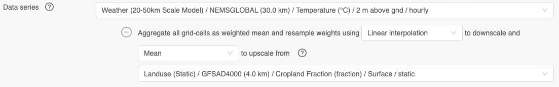
Again, grids both data-series must match or the transformation Aggregate all grid-cells as weighted mean and resample weights using {interpolation} to downscale and {aggregation} to upscale from {data-series} can be applied. The second data-series will be used as weights and prior resampled to match the grid.

This technique can be used to e.g. calculate the average temperature weighted by cropland fraction. In this way cells that have no cropland do not influence the mean temperature at all, cells with 30% cropland fraction will only have an influence of 30% etc. The working example for this is:

• Select temperature from any dataset (e.g. ERA5 or NEMSGLOBAL)
• Add the transformation Aggregate all grid-cells as weighted mean and resample
• Within the transformation select the dataset GFSAD4000 and the variable Cropland Fraction

Mask Out Grid Cells

The transformation Mask out grid-cells where value if {greater or less} {threshold} from {data series} can be used to set values to NaN. This can be used to only retrieve temperature data for grid-cells with a cropland fraction above 0.8. The masked-out grid-cells are not removed from the result, just set to NaN. This is important in case the transformation is combined with other transformations and must maintain a predictable behavior.

Similar to the previous transformations, the grid of both data-series must match. Otherwise the transformation Mask out grid-cells where (resampled) ... is applicable to match different dataset grids.

Downscale Grid Cells

For single location calls the API will select a best suitable nearest grid-cell. The best suitable might be the second closest, because the grid elevation might fit better. This is the recommended behavior. In rare cases it might be useful to interpolate between multiple grid-cells.

The transformation Downscale grid cells to location by interpolating between 3 triangulated neighbour grid cells will enable the interpolation between grid-cells. Internally this is an expensive operation, because it has to process a lot more data.